

I’d like to present a lesson by professor Ruggero Bertelli on the subject of deterministic statistical indicators as they compare to classic indicators of mean and variance.
LET’S SEE IT IN ACTION
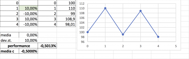
Assuming we have an investment that in the first year earned 10%, the following year lost 10%, the third year earned another 10% and the fourth year lost 10%, what would be the return on investment at the end of the four years?
THINK ABOUT YOUR ANSWER BEFORE YOU KEEP READING
If your answer was zero, perhaps you forgot that returns are not linear, and losses are not equal to the returns necessary to recover them. If I’ve lost 50%, to return to the initial value I would have to earn 100%. If I lost 10%, to get even, I’d have to make almost 11% back, as you can see from the image below.
At the four-year mark, I’d find myself with around 98 euros from the initial 100 I invested, with a real return of -0.5% per year and a volatility of 10%. The thing to note here is that the average of these returns is equal to zero, and if I have a historical series where the average = 0 it is likely that I actually lost some money.
LET’S GET A BIT MORE SERIOUS NOW
Using a different example, let’s take a random historical series where there is a 50% chance we could get a monthly return of +10% or -10% and we interrupt it after ten years when it’s measuring a positive overall return.
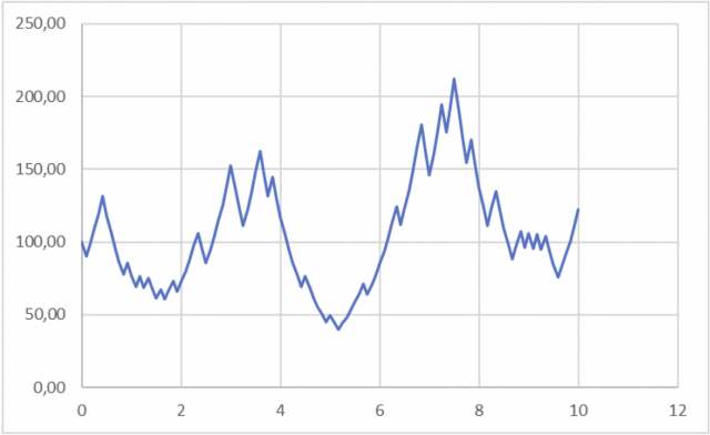
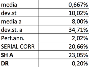
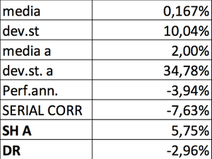
Looking at the data we’d notice a monthly average of 0.6% and a monthly volatility of 10%, and if we were to annualize those returns we’d have an average of 8% and volatility of 34%.In actuality, the historical series had an average annual return of just over 2%, certainly not 8%, which in 10 years would have more than doubled the capital.
The problem, as we can see from the table below, is that the Sharpe Ratio (“SH A”) is higher than 0.2 when in reality it would have been 0.05, almost zero. Vice versa, the DIAMAN Ratio (“DR”), explained in several instances including Introduction to the DIAMAN Ratio, Momentum Strategies using the DIAMAN Ratio, TIMING Strategy using the DIAMAN Ratio, due to it being quite a variable historical series, is low because there is no clear indication of future trends.
But if we were to take another random historical series and calculated it using the same random approach with returns of +10% and -10%, only in this case having a negative return at the end of the 10 years, the defects of the mean/variance indicators become obvious.
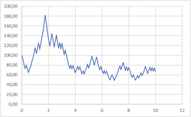
While the volatility remains practically the same with regards to the previous example for both monthly and yearly averages (a sign that the Montecarlo simulation engine has done its job), the monthly average is positive and consequently the annual average also seems decent (2% cannot be defined as a great return with a yearly mean volatility of 34%).
In reality, the average annual performance is negative at almost -4% per year, therefore quite a high loss in the end at the expense of a positive mean/variance, given that the Sharpe Ratio is even just slightly positive (0.05). The DIAMAN ratio proves to be a lot more consistent with reality, since it indicates an expected return of around -2.9% per year.
NOW LET’S REALLY GET SERIOUS
At this point, with an inquisitive spirit, Prof. Bertelli has carried out two Montecarlo simulations generating 10,000 historical series where the probability of having a return of +10% is 50% and the probability of obtaining a -10% is also 50%.
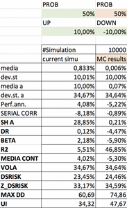
This simulation shows that the average of the 10,000 simulations is zero, the monthly volatility is still 10%, the annual is 34%, while the average real annual performance is at about -5%. The Sharpe Ratio is positive, while the negative part of the volatility, also known as Downside Volatility (“DSRISK”) is 24%. The DIAMAN Ratio (“DR”) correctly indicates a -4.47% return, therefore closest to reality, and the Ulcer Index (“UI”) has a value of 47.
FINAL SIMULATION
Now let’s look at another series of 10,000 Montecarlo simulations where I don’t tell you upfront which returns were positive or negative, and you can take a guess at how they might be configured in terms of positive or negative (always at 50% probability).
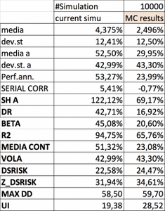
If we look at and understand volatility as a risk indicator instead of uncertainty, as I explained in the past, these 10,000 historical series, with an annualized volatility of 43% would appear much riskier than the previous ones.
QUESTION
The average return is positive, but is this positivity due to the increase in volatility or better yet to an asymmetry of positive and negative returns? From the mean/variance indicators it’s not at all easy to understand, but we can learn a lot of useful information if we look at the deterministic indicators (ie. DIAMAN Ratio, Ulcer Index, Downside Volatility and Drawdown). In fact, Downside Volatility is at 22%, which is slightly lower than the previous example despite the increase in volatility, showing a clear asymmetry.
DETERMINISTIC INDICATORS
The superiority of the deterministic indicators is evident not so much from the DIAMAN Ratio of 16% (which clearly reflects the uncertainty of the historical series, highlighted by the coefficient of determination R2 with a mean value of 67%), but by the Ulcer Index, which is much lower than in the previous example, highlighting that this second configuration of the Montecarlo simulation needs much less time to recover than the minimum time of the previous one.
These considerations, together with the articles Top 4 problems with the Sharpe Ratio – part 1 and The 4 main problems with the Sharpe Ratio – part 2 (available in this blog), are meant to put the indicator’s use into question. It’s not that the indicator itself is wrong, but rather our use of it. Nobel Prize winner William Sharpe himself pointed this out in a 1998 paper, titled “Morningstar’s Risk Adjusted Ratings”. The indicator was not created, nor is it useful for the selection of mutual funds.
ALWAYS LOOK FURTHER
Don’t believe it? Well, give yourself the time to read his paper and you’ll convince yourself without having to take me at my word, as one should always do when approaching such delicate issues as financial statistics.